Background
Since OpenAI introduced ChatGPT, large language models (LLMs) have gained significant attention and rapid development. Many enterprises are investing in LLM pre-training to keep up with this trend. However, training a 100B-scale LLM typically requires substantial computational resources, such as clusters equipped with thousands of GPUs. For example, the Falcon series model trains a 180B model on a 4096 A100 GPU cluster, taking nearly 70 days for 3.5T tokens. As data scales continue to grow, the demand for compute power increases. Meta, for instance, trained its LLaMA3 series model using 15T tokens across two 24K H100 clusters.
In this article, we delve into the components and configurations involved in building large-scale GPU clusters. We’ll cover different GPU types, server configurations, network devices (such as network cards, switches, and optical modules), and data center network topologies (e.g., 3-Tier, Fat-Tree). Specifically, we’ll explore NVIDIA’s DGX A100 SuperPod and DGX H100 SuperPod configurations, as well as common topologies used in multi-GPU clusters.
Keep in mind that constructing ultra-large GPU clusters is an extremely complex endeavor, and this article only scratches the surface. In practical cluster deployment, storage networks, management networks, and other aspects come into play, but we won’t delve into those details here. Additionally, network topology designs vary based on different application scenarios. Our focus will be on tree-based topologies commonly used in large-scale AI GPU clusters. Lastly, we won’t cover critical components like power systems and cooling systems, which are essential for maintaining and operating GPU clusters.
Relevant Components
GPUs
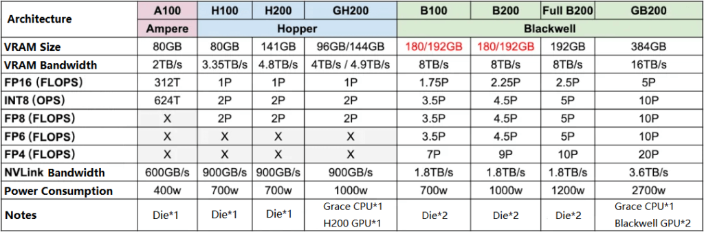
The chart below illustrates Ampere, Hopper, and the latest Blackwell series GPUs. Notice that memory capacity, computational power, and NVLink capabilities are gradually improving:
A100 -> H100: FP16 dense compute increases by over 3x, while power consumption only rises from 400W to 700W.
H200 -> B200: FP16 dense compute doubles, with power consumption increasing from 700W to 1000W.
B200 FP16 dense compute is approximately 7x that of A100, while power consumption is only 2.5x higher.
Blackwell GPUs support FP4 precision, offering twice the compute power of FP8. Some comparisons between FP4 and Hopper’s FP8 architecture show even more significant acceleration.
Note that GB200 uses the full B200 chip, while B100 and B200 are corresponding cut-down versions.
HGX Servers
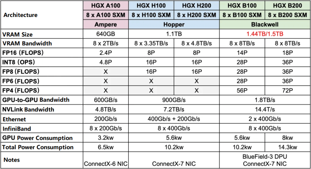
HGX is a high-performance server from NVIDIA, usually containing 8 or 4 GPUs, typically paired with Intel or AMD CPUs, and using NVLink and NVSwitch to achieve full interconnection (8 GPUs are usually the upper limit of NVLink full interconnection, except for NVL and SuperPod).
From HGX A100 -> HGX H100 and HGX H200, the FP16 dense computing power increased by 3.3 times, while the power consumption is less than 2 times.
From HGX H100 and HGX H200 -> HGX B100 and HGX B200, the FP16 dense computing power increased by about 2 times, while the power consumption is similar, at most not more than 50%.
It should be noted that:
The network of HGX B100 and HGX B200 has basically not been upgraded, and the IB network card is still 8x400Gb/s.
NVIDIA DGX and HGX are two high-performance solutions designed for deep learning, artificial intelligence, and large-scale computing needs. However, they differ in design and target applications:
DGX:
Targeted at general consumers.
Provides plug-and-play high-performance solutions.
Comes with comprehensive software support, including NVIDIA’s deep learning software stack, drivers, and tools.
Typically pre-built and closed systems.
HGX:
Targeted at cloud service providers and large-scale data center operators.
Suitable for building custom high-performance solutions.
Offers modular design, allowing customers to customize hardware based on their requirements.
Usually provided as a hardware platform or reference architecture.
Regarding networking:
Networking
Network Cards
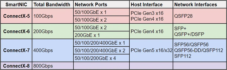
We’ll focus on ConnectX-5/6/7/8, which are high-speed network cards from Mellanox.
These cards support both Ethernet and InfiniBand (IB).
ConnectX-5 was released in 2016, followed by ConnectX-6 in 2020, ConnectX-7 in 2022, and ConnectX-8, which was introduced by Jensen Huang during the 2024 GTC conference (though detailed specifications are not yet available).
Each generation roughly doubles the total bandwidth, and the next generation is estimated to reach 1.6 Tbps.
Switches
NVIDIA also offers switches for both Ethernet and InfiniBand (IB). These switches often have dozens or even hundreds of ports, corresponding to a total throughput (Bidirectional Switching Capacity) calculated as the maximum bandwidth multiplied by the number of ports, with the “2” indicating bidirectional communication.
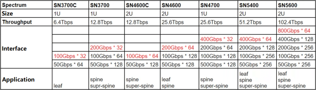
Spectrum-X Series Ethernet Switches
Quantum-X Series InfiniBand Switches:
These switches deliver 400 Gb/s throughput.
They excel in high-performance computing (HPC), AI, and hyperscale cloud infrastructures.
Quantum-X switches offer robust performance while minimizing complexity and cost.
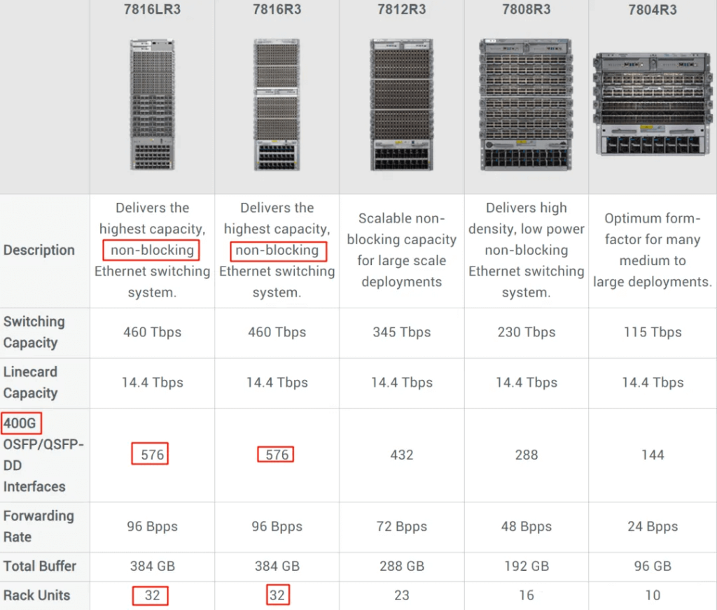
In addition to Mellanox switches, many data centers now adopt modular switches (such as the Arista 7800 series) alongside traditional options. For instance, Meta recently built two GPU clusters with 24K H100 GPUs, utilizing Arista 7800 switches. The 7800 series includes modular switches like the 7816LR3 and 7816R3, which can provide 576 ports of 400G high-speed bandwidth. These switches use efficient internal buses or switch backplanes for low-latency data transmission and processing.
Optical Modules
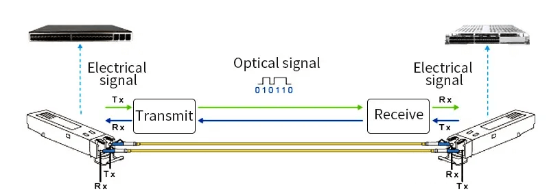
Optical modules play a crucial role in optical fiber communication. They convert electrical signals into optical signals, which are then transmitted through optical fibers. These modules offer higher transmission rates, longer distances, and greater immunity to electromagnetic interference. Typically, an optical module consists of a transmitter (for converting electrical to optical signals) and a receiver (for converting optical to electrical signals).
Two commonly used optical module interface types are:
SFP (Small Form-factor Pluggable): SFP modules usually operate as single transmission channels (using one fiber or a pair of fibers).
QSFP (Quad Small Form-factor Pluggable): QSFP modules support multiple transmission channels. QSFP-DD (Double Density) further enhances port density by using 8 channels.
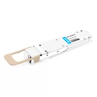
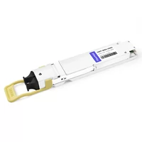
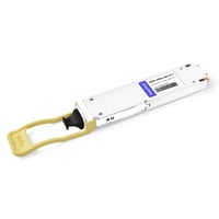
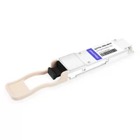
Recently, the OSFP (Octal Small Form-factor Pluggable) packaging has emerged, specifically designed for high-bandwidth scenarios like 400Gbps and 800Gbps. OSFP modules have 8 channels and are slightly larger than QSFP-DD. They are not compatible with SFP and QSFP interfaces and require converters. The diagram below illustrates 400Gbps OSFP modules for different transmission distances (100m, 500m, 2km, and 10km).
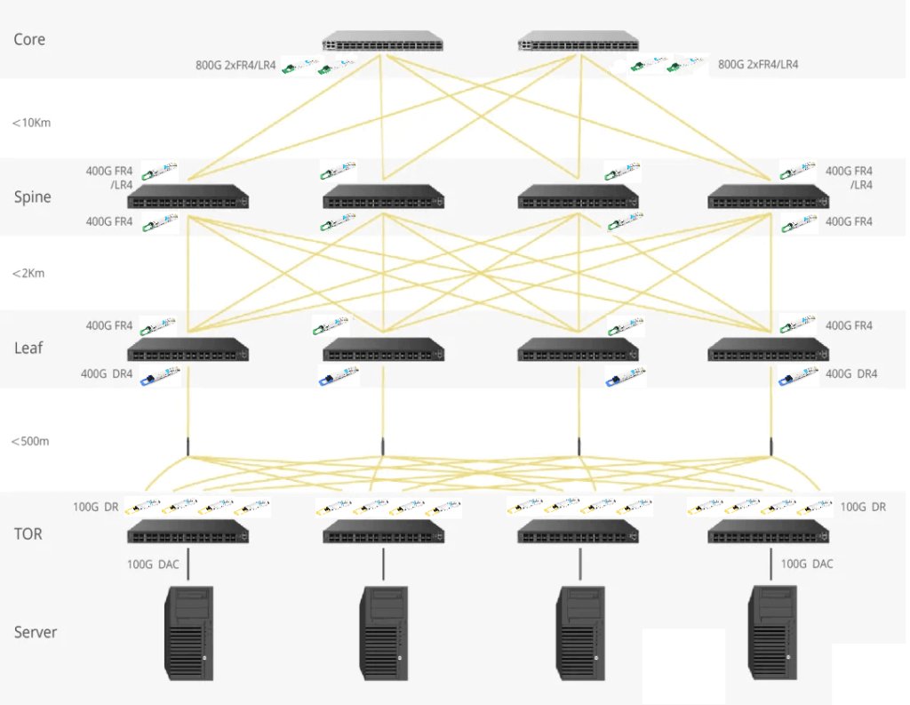
For various distances, consider the following module choices:
Between Core and Spine layers: Use 10km 400G LR4 or 800G 2xLR4.
Between Spine and Leaf layers: Opt for 2km 400G FR4.
Between Leaf and ToR (Top of Rack): Choose 500m 400G DR modules.
Data Center Network (DCN) Topology
Basic Concepts
North-South Traffic: Refers to traffic coming from outside the data center. It includes not only internet-related traffic but also traffic between different data centers.
East-West Traffic: Refers to traffic within the same data center. For example, it encompasses communication between different servers within the data center. In modern data centers, this type of traffic typically constitutes a significant portion, often accounting for 70% to 80% of the total.
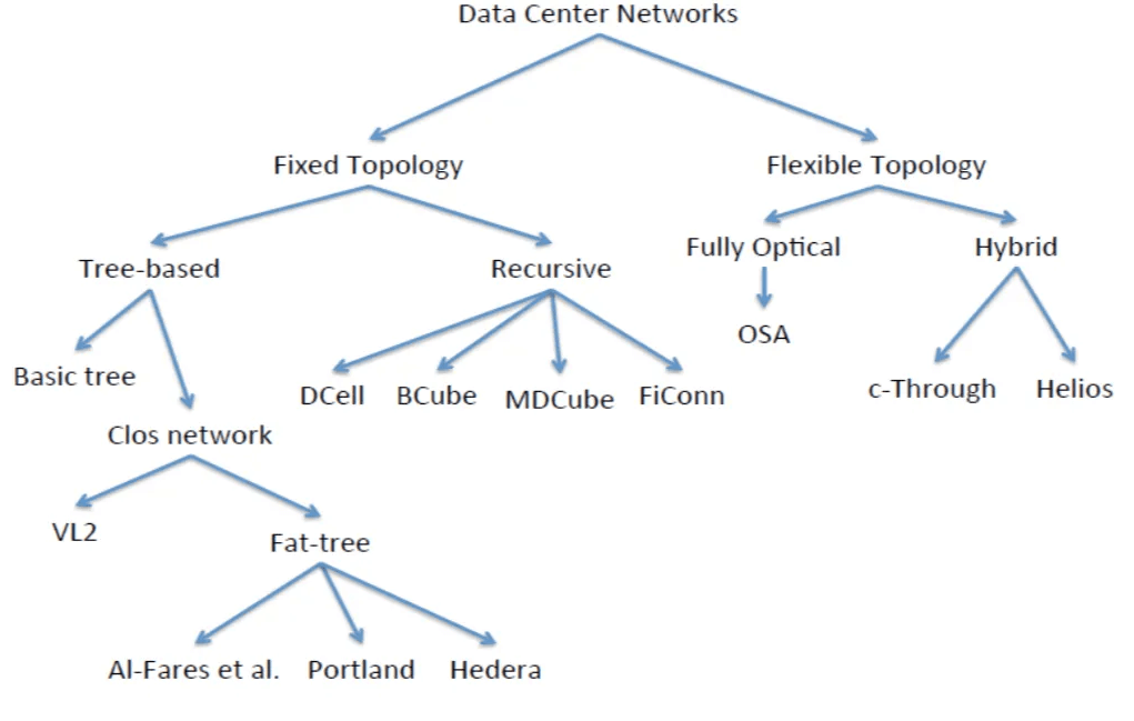
Common data center network (DCN) topologies are illustrated in the diagram below.
Multi-Tier DCN Architecture
Multi-tier DCN architectures are prevalent, especially the 3-tier DCN architecture. This tree-based structure primarily manages North-South traffic and consists of three layers:
- Core Layer: The core layer typically comprises high-capacity routers or switches.
- Aggregation Layer (Distribution Layer): Responsible for connecting access layer devices and providing routing, filtering, and traffic engineering between them.
- Access Layer: The access layer is where end-user devices connect directly to the network, facilitating the connection of user devices to the data center network.
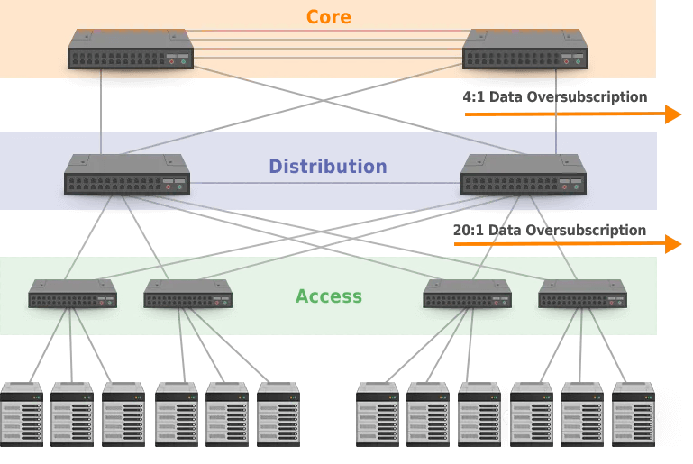
In this architecture, it is generally assumed that not all access devices communicate simultaneously at maximum bandwidth. Therefore, a common practice is to allocate smaller total bandwidth as we move up the hierarchy. For example, the total bandwidth at the access layer might be 20 Gbps, while the distribution layer’s total bandwidth could be only 1 Gbps. In extreme cases, if all devices communicate at maximum bandwidth, this can lead to blocking, increased latency, and unpredictable delays. This situation is often referred to as oversubscription, with the ratio (e.g., 20:1) indicating the oversubscription rate.
Within this architecture, redundancy or backup mechanisms are typically present. Switches between the core and distribution layers may interconnect, potentially creating loops. To avoid loops, spanning tree protocols (such as the Spanning Tree Protocol, STP) are used. However, this can also result in wasted bandwidth due to redundancy.
CLOS Networks
CLOS networks are a multi-stage switching network structure initially proposed by Charles Clos in 1953. Although originally used for telephone exchanges, their principles and design are now widely applied in data centers and high-performance computing. The core idea is to provide high bandwidth and low-latency network services through a multi-stage interconnected structure while maintaining scalability.
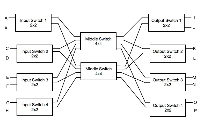
As shown in the diagram below, CLOS networks typically consist of three layers:
Ingress Layer: Responsible for receiving external input signals.
Middle Layer: Connects the ingress layer to the egress layer switches.
Egress Layer: Responsible for sending data to the final destination.
CLOS networks offer the following features and advantages:
Non-Blocking: Ideally, a CLOS network design is non-blocking (without convergence), meaning that data transmission delays or losses do not occur due to switch bottlenecks.
Scalability: By adding more layers and switches, CLOS networks can easily scale to support additional input and output connections without sacrificing performance.
Redundancy: The design’s multiple paths allow data to be transmitted via alternative routes even if certain switches or connections fail, enhancing overall network reliability.
Flexibility: CLOS networks support various configurations to accommodate different system sizes and performance requirements.
Fat-Tree Topology
The Fat-Tree data center network (DCN) architecture is a specialized form of the CLOS network. It is widely used in high-performance computing and large-scale data centers.
Charles Leiserson introduced this network topology in 1985. Unlike the traditional 3-tier tree networks, Fat-Tree topology has some unique features:
All layer switches are replaced with low-cost switches.
As we move upward in the hierarchy, the links “thicken,” maintaining consistent total bandwidth between layers to avoid bottlenecks.
The number of switches and their connections are symmetric at each layer, ensuring balanced paths for devices and minimizing single points of failure.
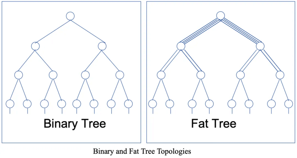
Maximizing End-to-End Bandwidth: The primary goal of Fat-Tree architecture is to maximize end-to-end bandwidth. It achieves a 1:1 oversubscription ratio, resulting in a non-blocking network.
Switch Count and Port Configuration:
In a K-port Fat-Tree network topology (where K is the number of ports per switch), all switches typically have the same number of ports.
Let’s explore the 2-layer and 3-layer Fat-Tree topologies:
2-Layer Fat-Tree Topology:
Spine Switches: K/2 switches, each with K*(K/2) ports.
Leaf Switches: K switches, each with K*K ports.
This configuration allows for a maximum of KK/2 servers in a non-blocking network, requiring 3K/2 network switches.
3-Layer Fat-Tree Topology:
Core Switches (Super Spine Switches): (K/2)^2 switches, each with K*(K/2)^2 ports.
Spine Switches: 2*(K/2)^2 switches, each with K2(K/2)^2 ports.
Leaf Switches: 2*(K/2)^2 switches, each with K2(K/2)^2 ports.
This design supports a maximum of K2(K/2)^2/2 = K^3/4 servers in a non-blocking network, requiring 5*K^2/4 switches.
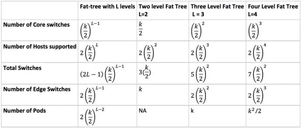
For both 2-layer and 3-layer Fat-Tree topologies, the switch counts and port configurations follow specific patterns.
Note that there are variations in terminology (e.g., Fat-Tree vs. Spine-Leaf), but we’ll consider them all under the Fat-Tree umbrella.
NVIDIA DGX SuperPod – A100
DGX A100 System
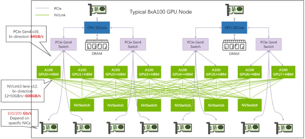
The DGX A100 System, as shown in the diagram below, is a 6U configuration with the following components:
8*A100 GPUs: Each GPU offers 600 GB/s NVLink bandwidth.
Total NVSwitch Bandwidth: The system achieves a total of 4.8 TB/s NVSwitch bandwidth, with 640 GB of HBM2 memory (80 GB per GPU).
Compute Connections (IB): There are 8 ConnectX-6 network cards, providing a combined total bandwidth of 8 * 200 Gbps.
Storage Connections (IB): 2 connections for storage.
In-Band Connection (Ethernet): Used for internal communication.
Out-Band Connection (Ethernet): For management purposes.
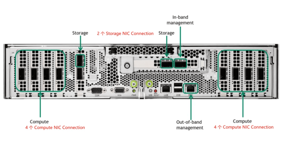
Notably, the NVLink bandwidth is measured in bytes, while network bandwidth typically uses bits. In this system, the internal bandwidth reaches 4.8 TB/s, whereas the overall network bandwidth is 1.6 Tbps, resulting in a 24-fold difference.
SuperPod SU
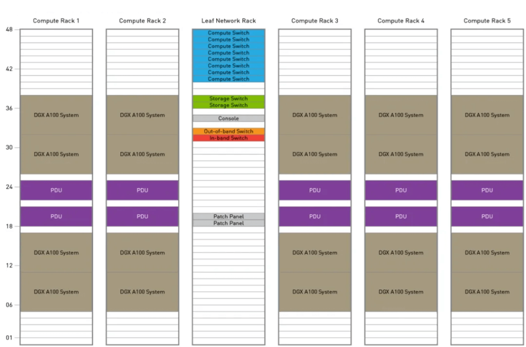
The SuperPod SU (Scalable Unit), depicted in the figure, serves as the fundamental building block for constructing the DGX-SuperPod-A100. Here are its key components:
Each SU includes 5 Compute Racks and 1 Leaf Network Rack.
Each Compute Rack houses 4 DGX A100 Systems and 2 3U Power Distribution Units (PDUs), totaling 32 A100 GPUs per Compute Rack. Thus, an SU comprises 160 A100 GPUs.
The Leaf Network Rack contains 8 Compute Switches (1U) and 2 Storage Switches (1U).
Compute Switches utilize QM8790 200 Gb/s IB switches, resulting in a total of 320 ports:
160 ports connect to the ConnectX-6 network cards in the Compute Racks, providing 200 Gbps per GPU.
The remaining 160 ports connect to the Spine Rack.
Some scenarios may also use Top-of-Rack (ToR) Switches within a cabinet for simpler cabling. However, this approach may lead to port wastage. For instance, due to power constraints and cooling challenges, GPU Servers are often limited to a single cabinet, reducing the number of network cards.
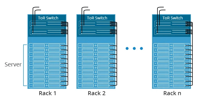
Please note that while some industrial scenarios may use fewer network cards (e.g., 4×200 Gbps) within an 8*A100 System, the overall network topology remains similar.
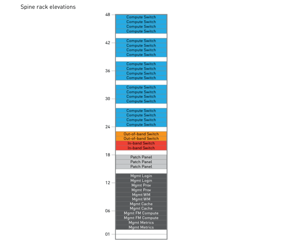
Spine Rack
As shown in the figure, a Spine Rack contains 20 1U Compute Switches, specifically QM8790 200 Gb/s IB switches, totaling 800 ports. The remaining Out-of-band Switch and In-band Switch can be used for network management.
DGX SuperPod 100-node
The figure below illustrates a 100-node DGX-SuperPOD, comprising 5 SUs and an additional Spine Rack.
Each SU includes 8 Leaf Compute Switches (QM7890, 200 Gbps).
Each Node’s 8 ConnectX-6 NICs connect to 8 Leaf Compute Switches, with each ConnectX-6 corresponding to 1 GPU.
The Leaf Compute Switches have 20 ports connecting to 20 Nodes within the SU, and an additional 20 ports connecting to the 20 Spine Compute Switches in the Spine Rack.
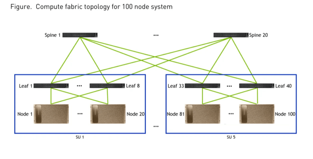
This topology achieves a non-blocking network for 800 GPUs (any two GPUs can communicate):
GPUs from different SUs connect via: ConnectX-6 -> Leaf Switch -> Spine Switch -> Leaf Switch -> ConnectX-6.
GPUs within the same SU but different Nodes connect via: ConnectX-6 -> Leaf Switch -> ConnectX-6.
GPUs within the same Node communicate via NVLink.
The practical limit for 800 GPUs (each GPU corresponding to a 200 Gbps NIC port) using QM8790 is a 2-level Fat-Tree network. Beyond 800 GPUs, a 3-level Fat-Tree would be needed, allowing up to 16,000 GPUs.
DGX SuperPod 140-node
In a 100-node system where all Compute Switch ports are occupied, expanding to more GPUs requires transitioning from 2-layer to 3-layer switches. This involves adding a Core Compute Switch layer, still using QM8790 at 200 Gbps.
Figure shows a 140-node SuperPod with 7 SUs, totaling 56 Leaf Switches. Ideally, 56 Leaf Switches would require 56 Spine Switches and 28 Core Switches. However, the actual design uses 80 Spine Switches, organized into 8 Groups (SG), each with 10 Spine Switches, and each Core Group (CG) with 14 Core Switches. This symmetric Fat-Tree topology simplifies management.
Each Leaf Switch in an SU connects to 10 Spine Switches in the corresponding SG (20 ports per Leaf Switch). Spine Switches alternate connections to Core Switches (odd positions to odd Core Switches, even positions to even Core Switches).
Each Core Switch connects to 40 Spine Switches.
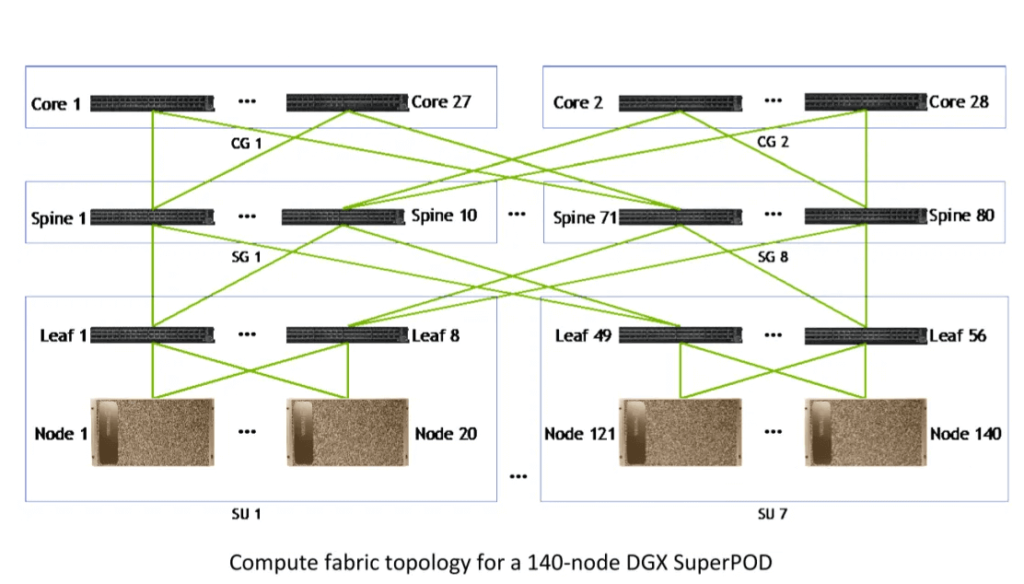
This configuration supports a 140*8=1120 GPU cluster, with each GPU having a ConnectX-6 200 Gbps NIC.
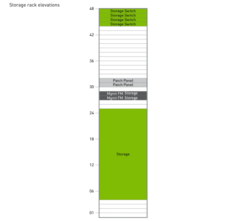
Storage Rack
As shown in the figure below, a Storage Rack contains 4 Storage Switches, also QM8790 200 Gbps IB switches, totaling 160 ports. The corresponding storage units are also present within the rack.
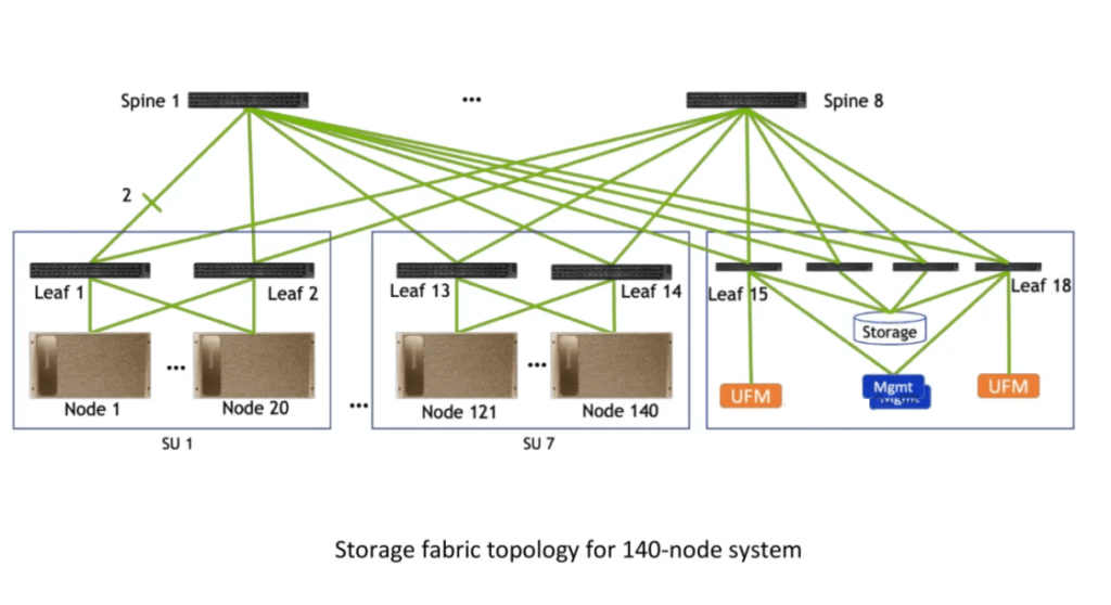
DGX SuperPod Storage Fabric
Figure illustrates the Storage Fabric for the 140-node configuration. It comprises 18 Leaf Switches. Each SuperPod SU (Scalable Unit) contains 2 Leaf Network Racks and 1 Storage Rack. Additionally, there are 8 Spine Switches.
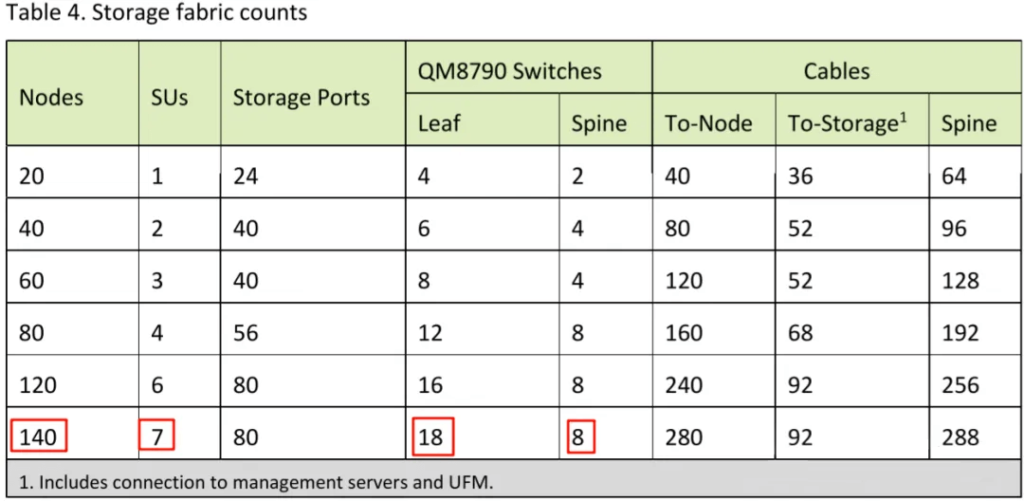
Additional Configurations
Table 3 provides details on the Compute configurations for different nodes.
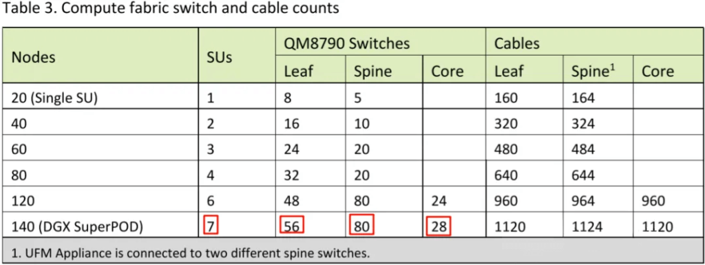
Table 4 outlines the Storage configurations.
NVIDIA DGX SuperPod – H100
DGX H100 System
The DGX H100 System (6U), as shown, includes:
- 8 H100 GPUs, each with 900 GB/s NVLink bandwidth.
- A total of 7.2 TB/s NVSwitch bandwidth and 640 GB HBM3 memory (80 GB per GPU).
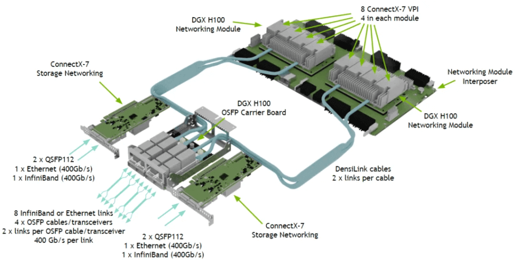
- 4 OSFP Ports (IB) corresponding to 8 ConnectX-7 NICs, providing 8*400 Gbps bandwidth.
- Slots 1 and 2 with 2 ConnectX-7 NICs, offering 2*400 Gbps bandwidth.
- An In-Band Connection (Ethernet).
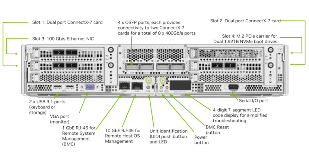
All 8 GPUs are fully interconnected via NVSwitch. The internal bandwidth reaches 7.2 TB/s, while the overall network bandwidth is 3.2 Tbps, a difference of 22.5 times.
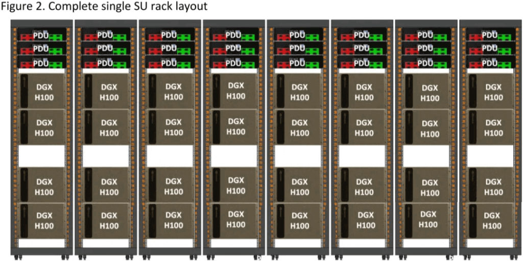
SuperPod SU
Figure 2 depicts the fundamental building block of the DGX-SuperPod-H100, known as the SuperPod SU:
- Each SU contains 8 Compute Racks, with each rack providing 40 kW.
- Each Compute Rack houses 4 DGX H100 Systems and 3 PDUs (Power Distribution Units), resulting in 32 H100 GPUs per Compute Rack. Thus, an SU accommodates 256 H100 GPUs.
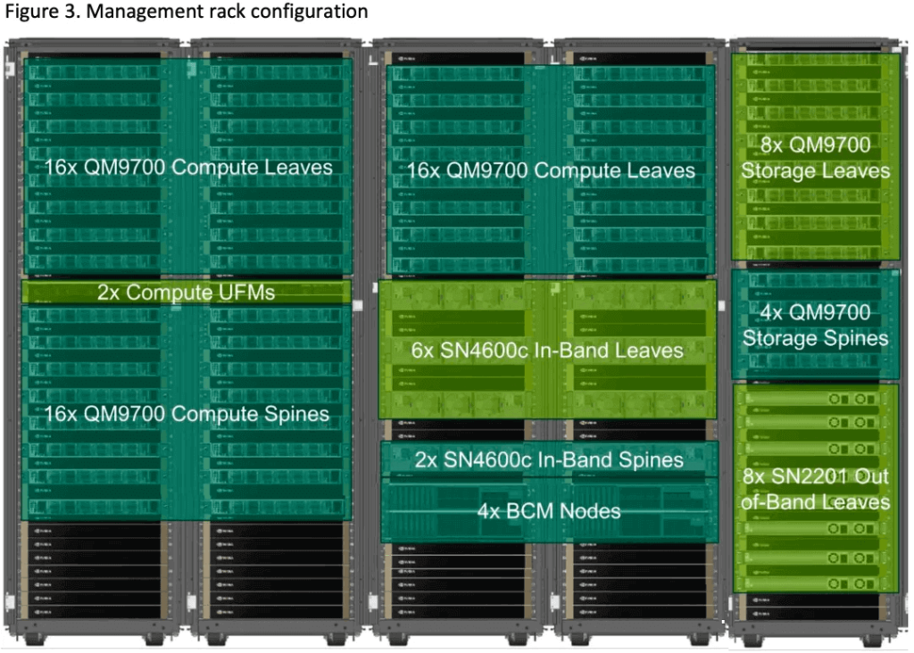
Management Rack
In the DGX SuperPod corresponding to H100 GPUs, NVIDIA offers a Management Rack similar to the A100 series’ Spine and Storage Racks. Figure 3 provides an example (specific configurations may vary):
- 32 Leaf Compute Switches (QM9700) offer 64 400 Gbps ports each. Theoretically, there are 1024 400 Gbps ports available to connect to the ConnectX-7 NICs on the nodes. The remaining 1024 ports connect precisely to 16 Spine Compute Switches, achieving a non-blocking network for 1024 GPUs.
- 16 Spine Compute Switches (also QM9700) connect to half of the ports on 32 Leaf Compute Switches.
- 8 Leaf Storage Switches (QM9700) are part of the setup.
- 4 Spine Storage Switches (QM9700) complete the configuration.
DGX SuperPod 127-node
Figure 5 illustrates a 127-node DGX SuperPod with 4 Scalable Units (SUs) and an associated Management Rack. In theory, the Management Rack can connect to the 128 nodes across the 4 SUs. However, due to some Leaf Switches being connected to the Unified Fabric Manager (UFM), the actual number of nodes is 127.
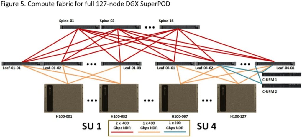
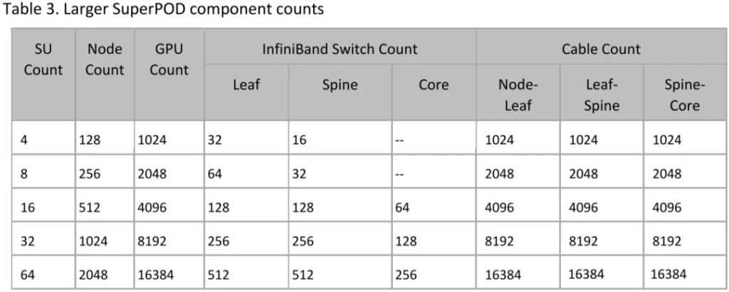
Additional Configurations
As shown in Table 3, using QM9700 switches, a 2-level Fat-Tree can achieve a non-blocking network for up to 6464/2=2048 GPUs (corresponding to 8 SUs). A 3-level Fat-Tree can support up to 6464*64/4=65536 GPUs. In practice, the configuration includes 64 SUs, totaling 16384 GPUs.
Industry GPU Training Cluster Solutions
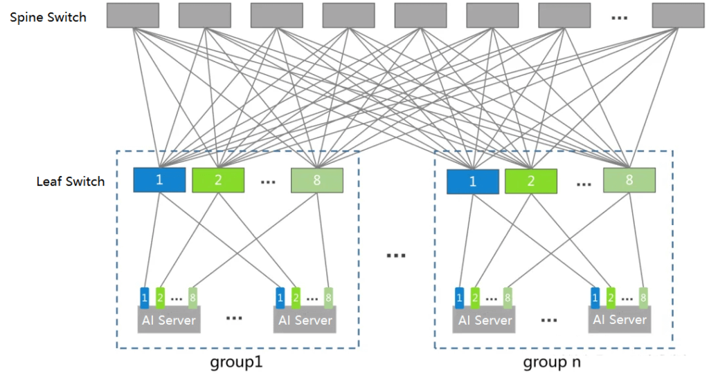
Two-Level Fat-Tree Topology
The common two-level non-blocking Fat-Tree topology (Spine-Leaf) is prevalent for 8-GPU training machines. Within a single machine, the 8 GPUs are fully interconnected via NVLink + NVSwitch, with communication bandwidth significantly higher than the network bandwidth. Therefore, it’s standard practice to connect each GPU’s NIC to different switches:
Each Group contains 8 Leaf Switches, corresponding to the 8 GPUs in a machine.
Assuming a Leaf Switch has 128 ports, 64 ports connect to the corresponding GPUs’ NICs, resulting in 64*8=512 GPUs per Group. Leaf Switch 1 connects all Node 1 GPUs’ NICs, and so on.
This feature can be leveraged when designing distributed training strategies.
To achieve Full Mesh between Spine and Leaf Switches, each Leaf Switch connects to one Spine Switch. Thus, there are 64 Spine Switches, and each Spine Switch connects to all 128 Leaf Switches. This requires 16 Groups.
In summary, a maximum of 192 switches with 128 ports each can support 512*16=8192 GPUs.
FiberMall Two-Level Fat-Tree Topology
The FiberMall standard solution for two-level Fat-Tree is similar to the previously described topology. However, it uses 64-port switches.
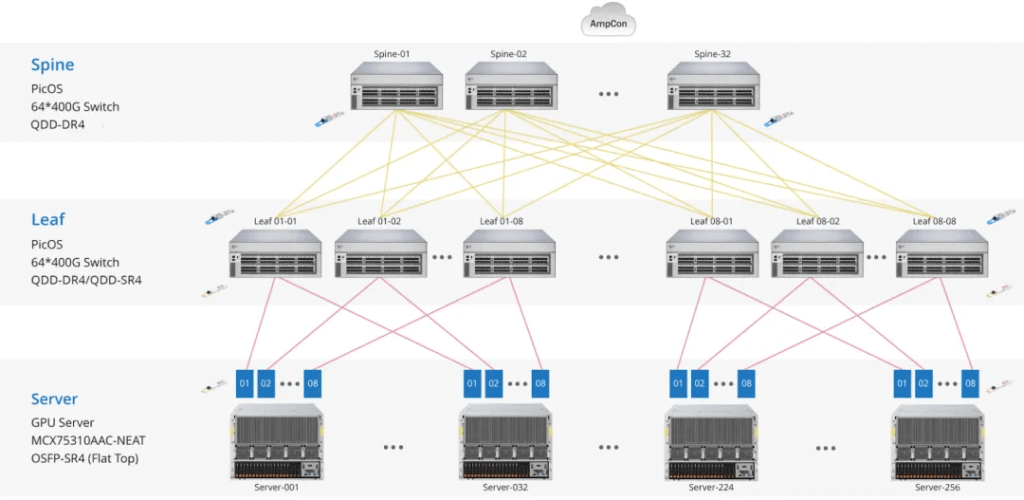
Due to the 64-port 400 Gbps switches:
Leaf and Spine Switches are halved (64 and 32, respectively).
GPU support reduces to 1/4, resulting in 2*(64/2)*(64/2)=2048 GPUs.
The total optical module count includes switch ports and GPU NICs: (64+32)*64+2048=8192.
Three-Level Fat-Tree Topology
The common three-level non-blocking Fat-Tree topology (SuperSpine-Spine-Leaf) treats the two-level Spine-Leaf as a Pod.
Since Spine Switches also connect to SuperSpine Switches, the number of Groups is halved. Each Pod has 64 Spine Switches, corresponding to 4096 GPUs.
Multiple Pods can further build 64 SuperSpine Fabrics, each fully interconnected with Spine Switches from different Pods. For example, with 8 Pods, each Fabric needs only 4 128-port SuperSpine Switches.
The configuration for 8 Pods includes:
- Total GPUs: 4096*8=32768
- SuperSpine Switches: 64*4=256
- Spine Switches: 64*8=512
- Leaf Switches: 64*8=512
- Total Switches: 256+512+512=1280
- Total optical modules: 1280*128+32768=196608
The theoretical maximum supports 128 Pods, corresponding to:
- GPUs: 4096128=524288=2(128/2)^3
- SuperSpine Switches: 64*64=4096=(128/2)^2
- Spine Switches: 64128=8192=2(128/2)^2
- Leaf Switches: 64128=8192=2(128/2)^2
- Total Switches: 4096+8192+8192=20480=5*(128/2)^2
Related Products:
-
 NVIDIA MMA4Z00-NS400 Compatible 400G OSFP SR4 Flat Top PAM4 850nm 30m on OM3/50m on OM4 MTP/MPO-12 Multimode FEC Optical Transceiver Module
$550.00
NVIDIA MMA4Z00-NS400 Compatible 400G OSFP SR4 Flat Top PAM4 850nm 30m on OM3/50m on OM4 MTP/MPO-12 Multimode FEC Optical Transceiver Module
$550.00
-
NVIDIA MMA4Z00-NS-FLT Compatible 800Gb/s Twin-port OSFP 2x400G SR8 PAM4 850nm 100m DOM Dual MPO-12 MMF Optical Transceiver Module
$650.00
-
NVIDIA MMA4Z00-NS Compatible 800Gb/s Twin-port OSFP 2x400G SR8 PAM4 850nm 100m DOM Dual MPO-12 MMF Optical Transceiver Module
$650.00
-
NVIDIA MMS4X00-NM Compatible 800Gb/s Twin-port OSFP 2x400G PAM4 1310nm 500m DOM Dual MTP/MPO-12 SMF Optical Transceiver Module
$900.00
-
NVIDIA MMS4X00-NM-FLT Compatible 800G Twin-port OSFP 2x400G Flat Top PAM4 1310nm 500m DOM Dual MTP/MPO-12 SMF Optical Transceiver Module
$1199.00
-
NVIDIA MMS4X00-NS400 Compatible 400G OSFP DR4 Flat Top PAM4 1310nm MTP/MPO-12 500m SMF FEC Optical Transceiver Module
$700.00
-
NVIDIA(Mellanox) MMA1T00-HS Compatible 200G Infiniband HDR QSFP56 SR4 850nm 100m MPO-12 APC OM3/OM4 FEC PAM4 Optical Transceiver Module
$139.00
-
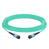
NVIDIA MFP7E10-N010 Compatible 10m (33ft) 8 Fibers Low Insertion Loss Female to Female MPO Trunk Cable Polarity B APC to APC LSZH Multimode OM3 50/125
$47.00
-
NVIDIA MCP7Y00-N003-FLT Compatible 3m (10ft) 800G Twin-port OSFP to 2x400G Flat Top OSFP InfiniBand NDR Breakout DAC
$260.00
-
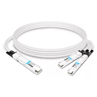
NVIDIA MCP7Y70-H002 Compatible 2m (7ft) 400G Twin-port 2x200G OSFP to 4x100G QSFP56 Passive Breakout Direct Attach Copper Cable
$155.00
-
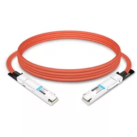
NVIDIA MCA4J80-N003-FTF Compatible 3m (10ft) 800G Twin-port 2x400G OSFP to 2x400G OSFP InfiniBand NDR Active Copper Cable, Flat top on one end and Finned top on other
$600.00
-
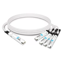
NVIDIA MCP7Y10-N002 Compatible 2m (7ft) 800G InfiniBand NDR Twin-port OSFP to 2x400G QSFP112 Breakout DAC
$190.00